
深度学习-pytorch-自动求导与线性回归
自动求导尝试
torch.Tensor 是这个包的核心类。如果设置它的属性 .requires_grad 为 True,那么它将会追踪对于该张量的所有操作。当完成计算后可以通过调用 .backward(),来自动计算所有的梯度。这个张量的所有梯度将会自动累加到.grad属性.
要阻止一个张量被跟踪历史,可以调用 .detach() 方法将其与计算历史分离,并阻止它未来的计算记录被跟踪。
为了防止跟踪历史记录(和使用内存),可以将代码块包装在 with torch.no_grad(): 中。在评估模型时特别有用,因为模型可能具有 requires_grad = True 的可训练的参数,但是我们不需要在此过程中对他们进行梯度计算。
还有一个类对于autograd的实现非常重要:Function。
Tensor 和 Function 互相连接生成了一个无圈图(acyclic graph),它编码了完整的计算历史。每个张量都有一个 .grad_fn 属性,该属性引用了创建 Tensor 自身的Function(除非这个张量是用户手动创建的,即这个张量的 grad_fn 是 None )。
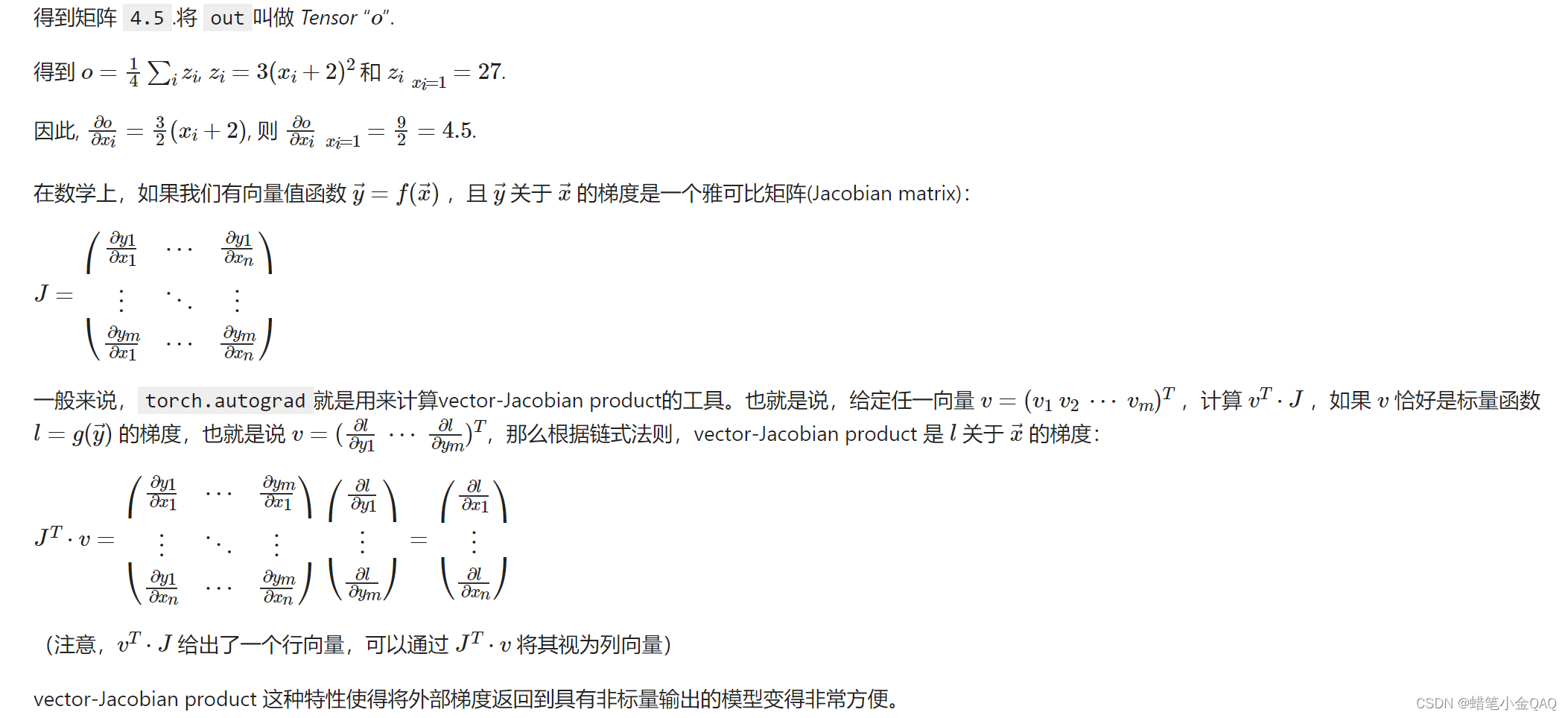
如果需要计算导数,可以在 Tensor 上调用 .backward()。如果 Tensor 是一个标量(即它包含一个元素的数据),则不需要为 backward() 指定任何参数,但是如果它有更多的元素,则需要指定一个 gradient 参数,该参数是形状匹配的张量。
1 | import torch |
1 | x = torch.ones(3, 2, requires_grad=True) |
tensor([[1., 1.],
        [1., 1.],
        [1., 1.]], requires_grad=True)
tensor([[3., 3.],
        [3., 3.],
        [3., 3.]], grad_fn=<AddBackward0>)
1 | x = torch.randn((2, 3), requires_grad=True) |
tensor([[-1.5443, -0.0354, -0.8403],
        [ 1.5566,  0.7182,  1.5884]], requires_grad=True)
tensor([[0.4557, 1.9646, 1.1597],
        [3.5566, 2.7182, 3.5884]], grad_fn=<AddBackward0>)
tensor([[1., 1., 1.],
        [1., 1., 1.]])
tensor(1720.7292, grad_fn=<MulBackward0>)
线性回归理解
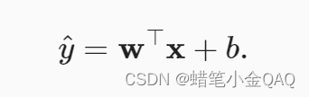
给定一个数据集,我们的目标是寻找模型的权重和偏置, 使得根据模型做出的预测大体符合数据里的真实价格。 输出的预测值由输入特征通过线性模型的仿射变换决定,仿射变换由所选权重和偏置确定。
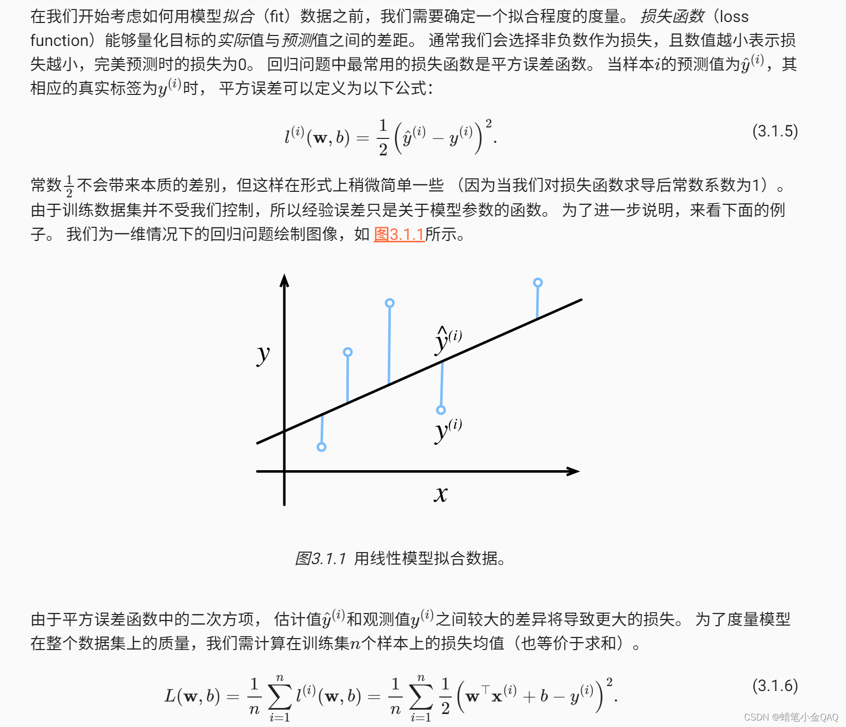
损失函数
线性回归的从零开始实现
其中d2l包需要自己导入离线安装,附上链接:感谢SWY大神
顺便补一个d2l_zh的包:再次感谢SWY大神
1 | from d2l import torch as d2l # 李沐大神自己写的包,需要自己导入 |
Using matplotlib backend: QtAgg
1 | def synthetic_data(w, b, num_examples): |
1 | print('features', features[0]) |
features tensor([-0.3295, -0.7524])
labels tensor([6.0904])
读取小批量
1 | def data_iter(batch_size, features, labels): # batch_size 批量大小 |
我们直观感受一下小批量运算:读取第一个小批量数据样本并打印。 每个批量的特征维度显示批量大小和输入特征数。 同样的,批量的标签形状与batch_size相等。
1 | batch_size = 10 |
tensor([[ 0.7996,  0.4114],
        [ 0.0760,  1.0155],
        [ 0.6860,  0.2270],
        [-2.0028,  0.9113],
        [ 0.4199, -0.6192],
        [-0.0252,  2.0244],
        [ 1.7162, -0.4195],
        [ 0.6579, -0.3955],
        [-1.5817, -0.1407],
        [-1.0975,  0.1836]])
 tensor([[ 4.4066],
        [ 0.8990],
        [ 4.8128],
        [-2.8907],
        [ 7.1436],
        [-2.7258],
        [ 9.0706],
        [ 6.8511],
        [ 1.5068],
        [ 1.3921]])
初始化模型参数
1 | w=torch.normal(0,0.01,size=(2,1),requires_grad=True) |
定义模型
1 | def linreg(X, w, b): |
定义损失函数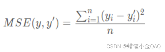
1 | def squared_loss(y_hat, y): |
定义优化算法
1 | def sgd(params, lr, batch_size): |
开始训练
另外附上python特有的print(f’’)用法:传送门
1 | lr = 0.03 # 学习率是0.03(太小效率太低,太大容易超出范围,造成摆动) |
epoch 1, loss 0.038161
epoch 2, loss 0.000139
epoch 3, loss 0.000048
输出通过学习修正过的参数值,评估训练成功程度
1 | print(f'w的估计误差: {true_w - w.reshape(true_w.shape)}') |
w的估计误差: tensor([ 0.0002, -0.0004])
b的估计误差: tensor([-0.0006])
tensor([[ 1.9998, -3.3996]])
tensor([4.2006])
线性回归深度学习框架的简洁实现
使用pytorch的nn来实现加载数据
1 | import numpy as np |
创建初始w,b。
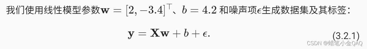
并且生成标签数据集
1 | true_w =torch.tensor([2,-3.4]) |
构造pytorch迭代器
1 | def load_array(data_arrrays, batch_size, is_train=True): |
[tensor([[ 0.1652,  0.8560],
         [ 0.0147,  1.5673],
         [ 0.9652, -0.2222],
         [ 0.4242,  0.1483],
         [ 0.8722, -1.3510],
         [ 0.0506,  0.8717],
         [-1.2767, -0.0087],
         [-0.4736,  0.8434],
         [-0.1852, -0.9320],
         [-1.6329,  0.1184]]),
 tensor([[ 1.6253],
         [-1.0980],
         [ 6.8757],
         [ 4.5338],
         [10.5444],
         [ 1.3342],
         [ 1.6711],
         [ 0.3882],
         [ 7.0090],
         [ 0.5239]])]
使用深度学习框架定好的层
1 | # nn是神经网络的缩写 |
初始化模型参数
1 | net[0].weight.data.normal_(0,0.01) #使用正太分布替换它的值,均值0,方差0.01 |
计算均方误差(平方范数)
1 | loss=nn.MSELoss() |
实例化SGD实例(优化算法)
1 | trainer = torch.optim.SGD(net.parameters(), lr=0.03) |
开始训练
回顾一下:在每个迭代周期里,我们将完整遍历一次数据集(train_data), 不停地从中获取一个小批量的输入和相应的标签。 对于每一个小批量,我们会进行以下步骤:
通过调用net(X)生成预测并计算损失l(前向传播)。
通过进行反向传播来计算梯度。
通过调用优化器来更新模型参数。
为了更好的衡量训练效果,我们计算每个迭代周期后的损失,并打印它来监控训练过程。
1 | num_epochs = 3 # 训练三次 |
epoch 1, loss 0.000246
epoch 2, loss 0.000098
epoch 3, loss 0.000098
输出并评估训练结果
下面我们比较生成数据集的真实参数和通过有限数据训练获得的模型参数。 要访问参数,我们首先从net访问所需的层,然后读取该层的权重和偏置。 正如在从零开始实现中一样,我们估计得到的参数与生成数据的真实参数非常接近
1 | w = net[0].weight.data |
w的估计误差: tensor([ 0.0002, -0.0004])
b的估计误差: tensor([-0.0006])
tensor([[ 1.9998, -3.3996]])
tensor([4.2006])